
Examples
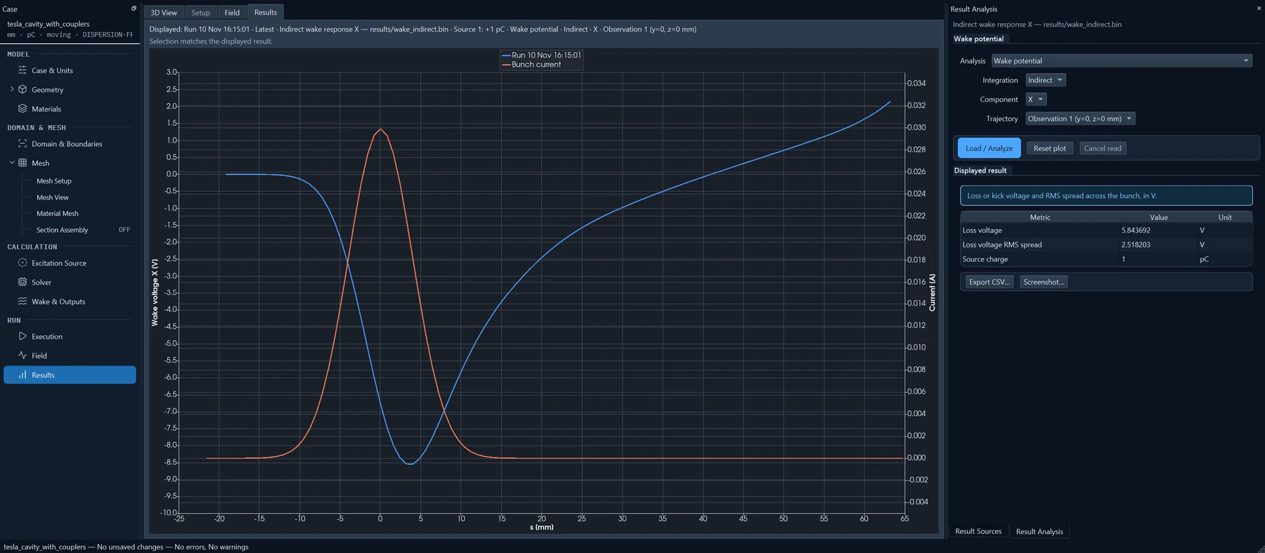
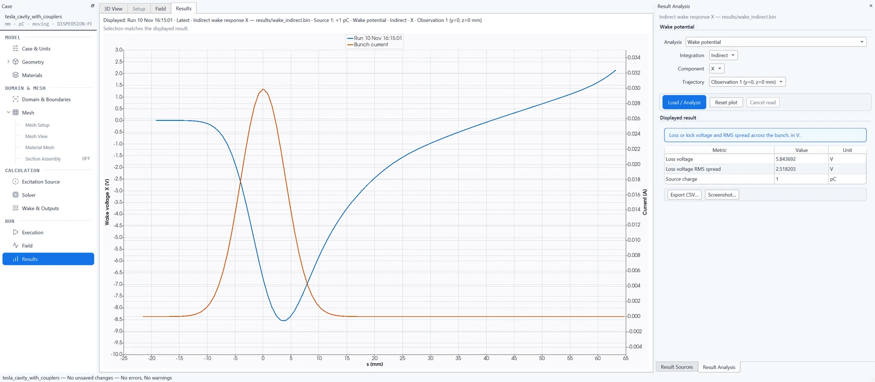
Four cases computed with EMUZAG. Each shows the model as Studio draws it, the field inside the section of its structure, the wake potential from Studio, and the settings of the run; for the pillbox, whose point is material loss, the text lists what Studio reports. Fields are played from the recorded solver output, one at a time. The Examples Guide describes the eight models that come with the package.
TESLA cavity with couplers
3D Solver
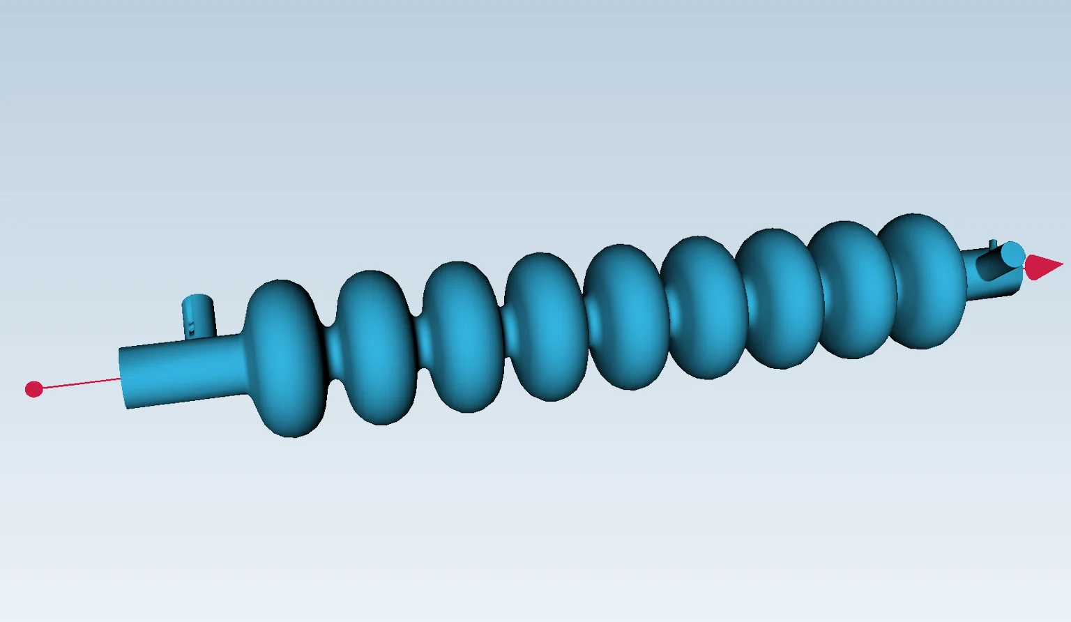
The superconducting 1.3 GHz nine-cell cavity with its couplers, imported as the vacuum volume.
- Bunch: 1 pC Gaussian, σ = 4 mm, β = 1, on axis.
- Field below: stationary grid, dispersion-free scheme, mesh 1.6 × 2.38 × 2.38 mm, EMUZAG 1.1.2.
- Wake: moving window, 0.8 mm mesh, 1,709 steps; 64 s of solver time on 6 MPI processes of an 8-core desktop PC, the largest process using 96 MB (3D Solver 1.2.0, pre-release).
- The 2D Solver, on the same cavity without couplers, gives a bunch loss 1.4 % away.
A moving window is a short mesh that travels with the bunch, so that only the field around and behind the bunch is computed.
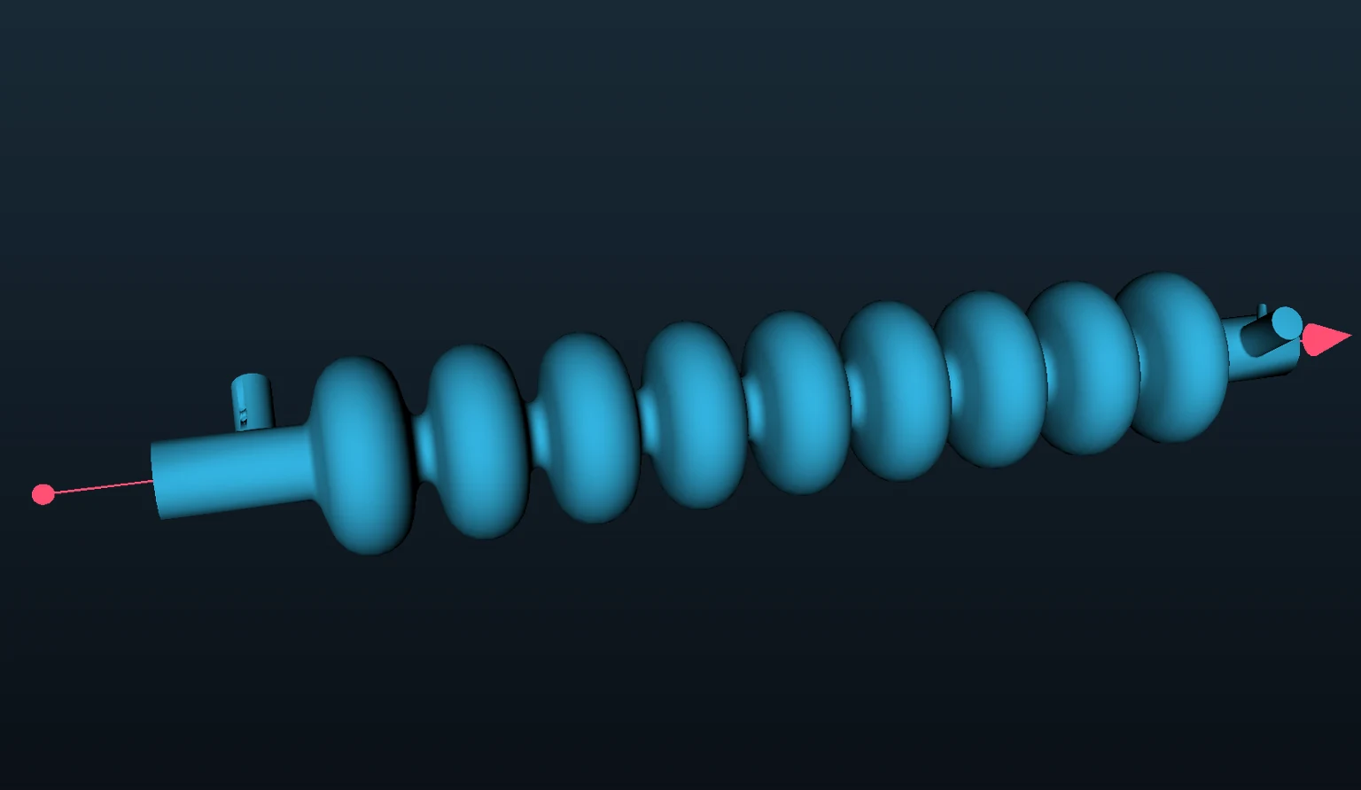
Field Ex on the plane through the beam axis, shown until about 520 mm after the bunch has left the cavity; red is positive, blue negative. The small islands near the ends are the couplers cut by the plane.
Tapered collimator
3D Solver
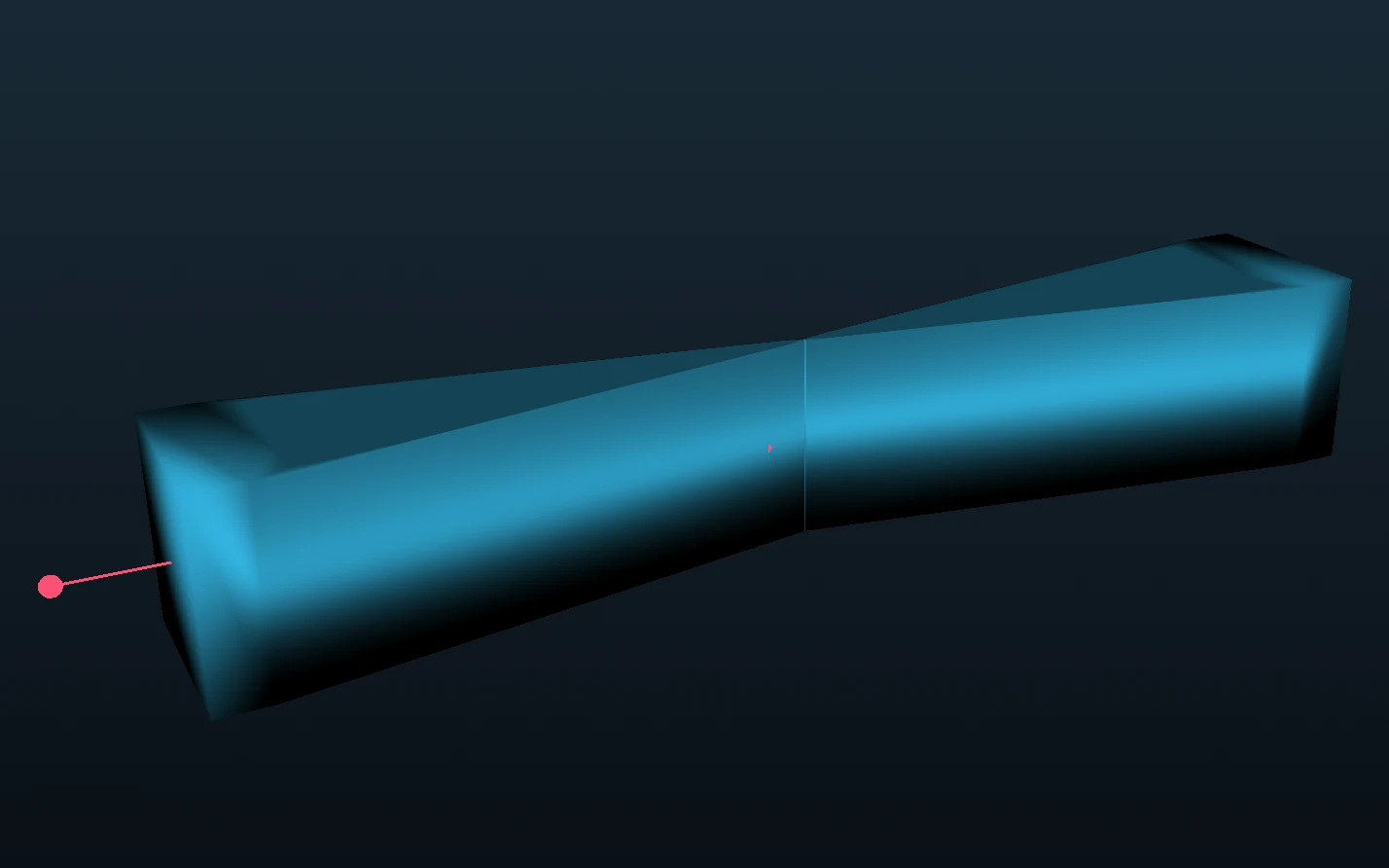
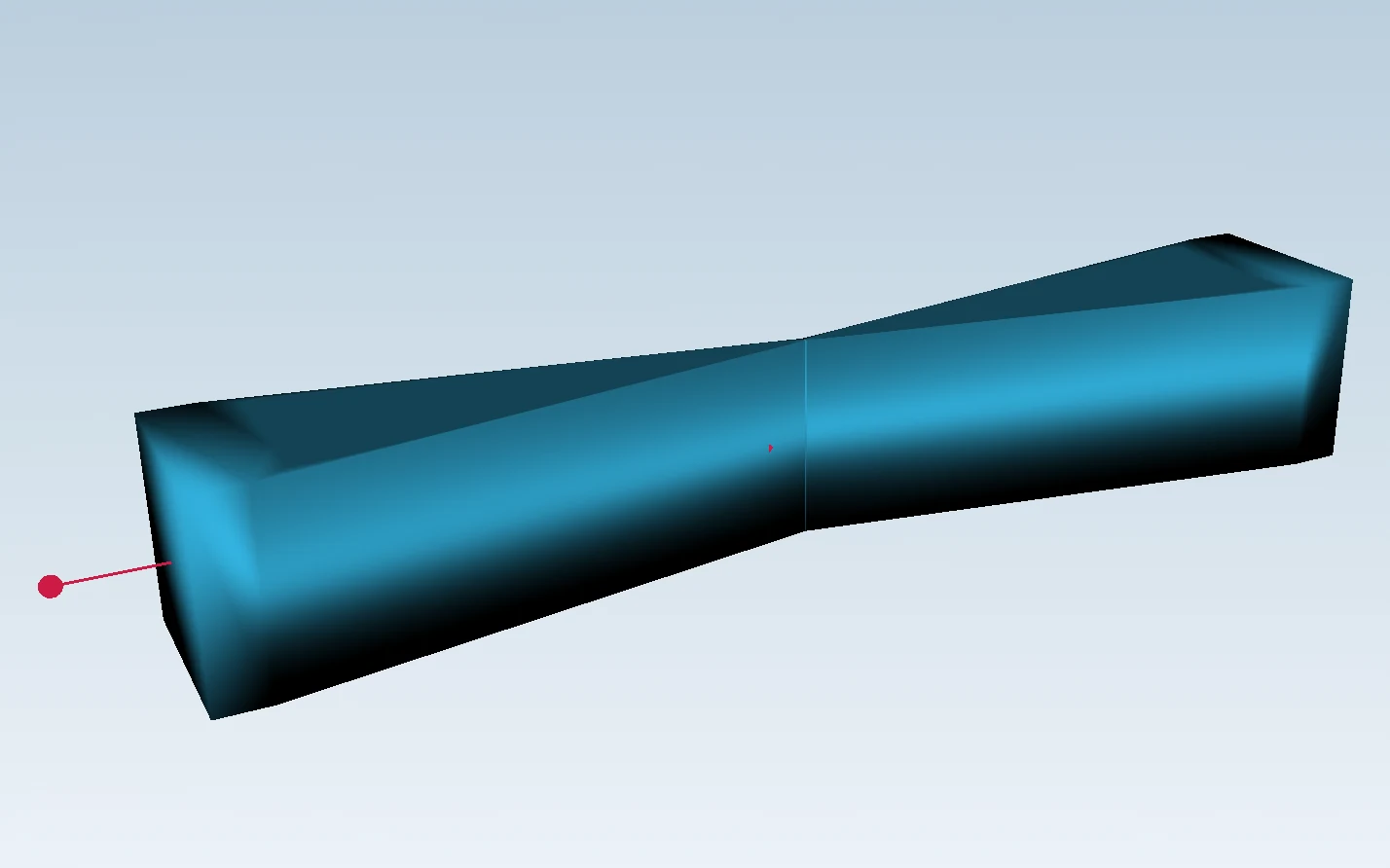
A rectangular collimator whose gap narrows from 38 mm to 1.4 mm over 104 mm and opens again. The Quick Start guide begins with this model.
- Bunch: 1 pC Gaussian, σ = 1 mm, β = 1, on axis.
- Stationary grid, dispersion-free scheme, mesh 0.2 × 0.297 × 0.297 mm, EMUZAG 1.1.2.
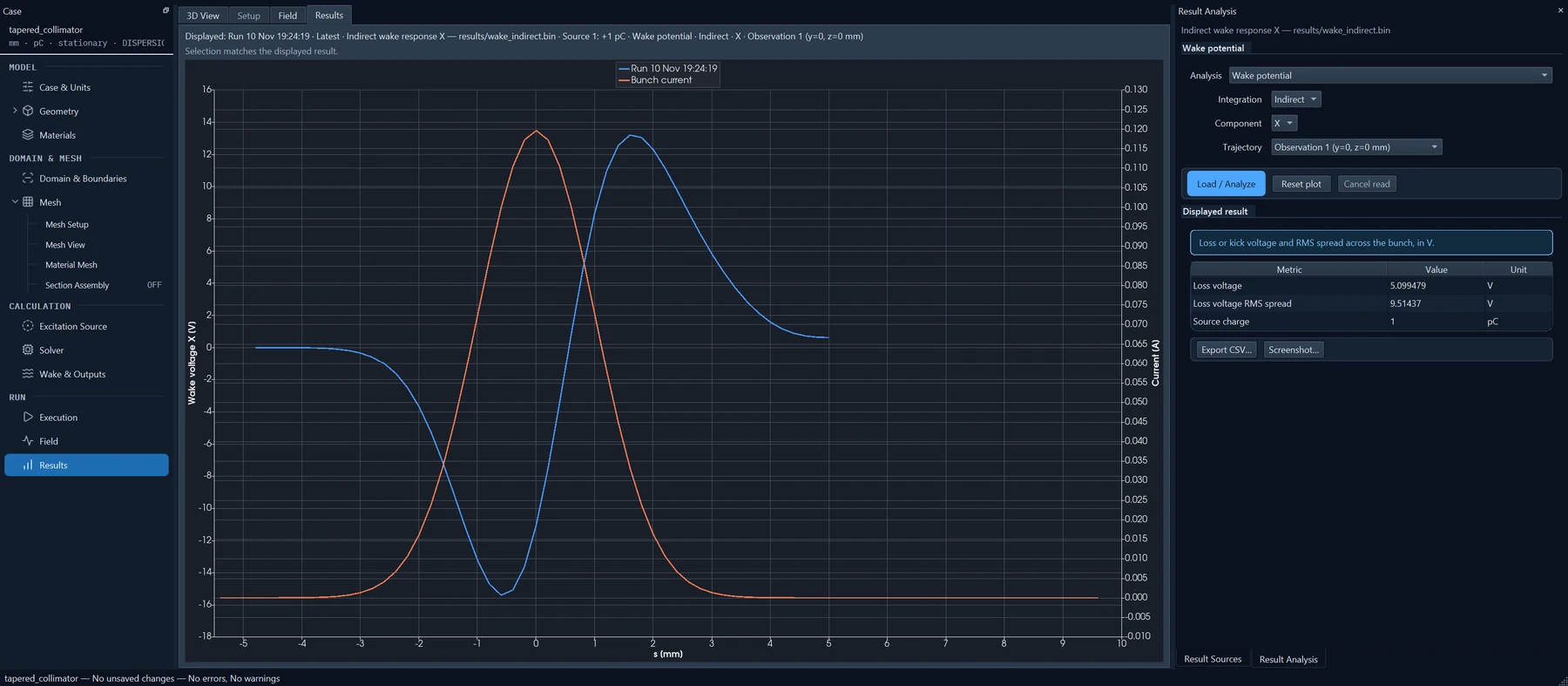
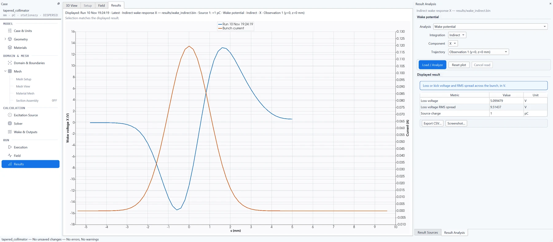
- Longitudinal wake potential by indirect integration.
Field Ex on the plane through the beam axis. Colour strength is compressed so the weak wake behind the bunch stays visible next to the bunch’s own field.
Corrugated pipe
2D Solver
A round corrugated pipe as a demonstration model: 48 periods of 0.5 mm with grooves 0.25 mm wide and 0.5 mm deep, an aperture radius of 2 mm, cones to a beam pipe of 4 mm radius, 44 mm in all.
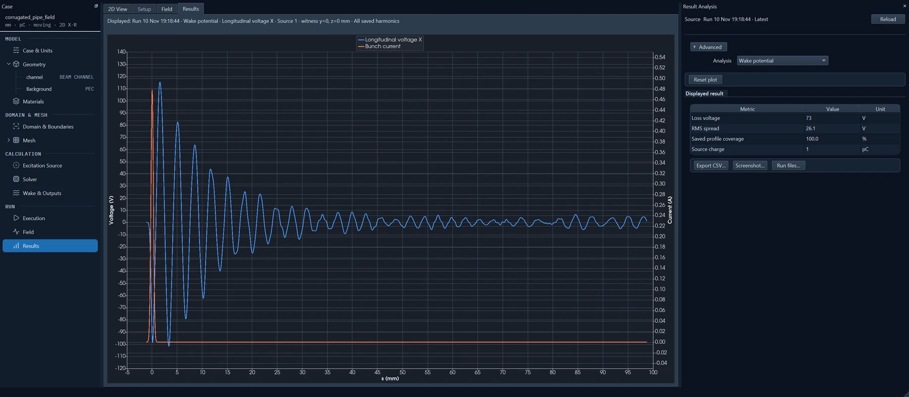
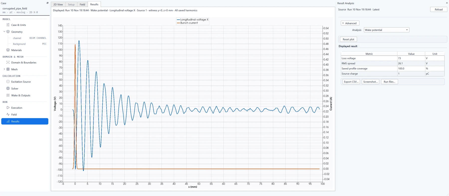
- Bunch: 1 pC Gaussian, σ = 0.25 mm. The field below is the monopole run with the bunch on the axis; the timed run has the bunch 0.5 mm off axis, with azimuthal harmonics m = 0 and 1.
- Moving window, 79,200 cells of 0.05 mm, 2,883 steps; 18–19 s on 6 threads (2D Solver 0.1.0, development build).
- The monopole line lies at 91 GHz; the small-corrugation estimate is 95 GHz.
A moving window is a short mesh that travels with the bunch, so that only the field around and behind the bunch is computed.
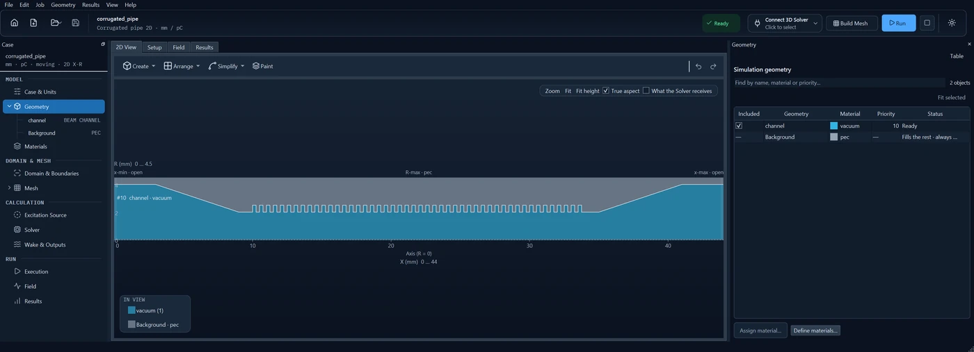
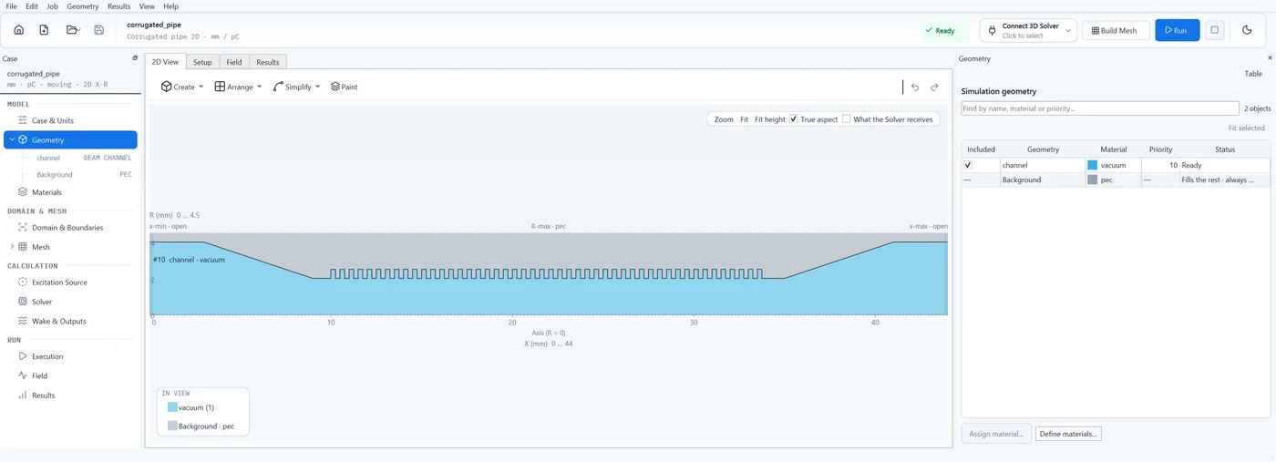
Field Ex of the monopole run with the bunch on the axis, in the plane of axis and radius; the half above the axis is computed and mirrored for the picture. The wake keeps ringing in the grooves after the bunch has passed.
Lossy pillbox
3D Solver, material losses
A pillbox cavity with copper walls (5.8 × 10⁷ S/m, surface-impedance model) and a lossy dielectric ring (εr = 4, 2 S/m); the example for material power loss. Studio reports the power lost in the copper wall and in the dielectric ring, per material and over time, with the cumulative loss.
- Bunch: 1 pC Gaussian, σ = 0.5 mm, β = 1, on axis.
- Stationary grid, dispersion-free scheme, mesh 0.1 × 0.148 × 0.148 mm, EMUZAG 1.1.2.
Field Ex on the plane through the beam axis, for the first 106 mm of bunch travel.