
The 2D Solver and the 3D Solver
EMUZAG computes wake potentials, impedances and material losses of accelerator components with dedicated 2D and 3D time-domain solvers. Models are prepared, run and analysed in one application, EMUZAG Studio.
2D Solver
Axisymmetric (X–R) and fixed-width planar (X–Z) structures. Azimuthal or width harmonics give off-axis excitation and transverse wakes on a 2D mesh. Saved modal coefficients evaluate new source and witness offsets without a new field calculation. Runs as one process with OpenMP threads on a workstation.
Free for non-profit research and teaching organisations. Registration opens when the academic licence terms are published; until then, write to the team from an institutional email address.
3D Solver
General three-dimensional geometry on a conformal Cartesian mesh. Stationary and moving-window time-domain methods, longitudinal and transverse wakes, several synchronous sources, conducting walls and coatings, electric and magnetic dispersion, beams below the speed of light on stationary grids, and two-port multimode S-parameters. Hybrid MPI and OpenMP on workstations and clusters.
Licensed. Evaluation licence on request; commercial and academic licences by quotation.
EMUZAG Studio
One application for 2D and 3D projects: geometry and CAD import, meshing, solver setup and run control, field playback, wake and impedance analysis, resonance fitting and material-loss reports.
No licence needed. Desktop application for Windows x64 and macOS on Apple Silicon. Comes with every package.
Capabilities side by side
| 2D SolverFree for non-profit research and teaching organisations | 3D SolverLicensed | |
|---|---|---|
| Model | ||
| Geometry | Axisymmetric (X–R); fixed-width planar (X–Z), symmetric or asymmetric | General 3D: STEP/BREP, STL, or built in Studio |
| Mesh | Conformal, in the two solved coordinates | Conformal Cartesian |
| Methods | ||
| Moving window (β = 1) | Dispersion-free TE/TMboth solvers | |
| Stationary grid | Implicit dispersion-free; FDTD in selected workflows | Explicit and implicit dispersion-free; FDTD |
| Beams with β < 1 | Selected stationary workflows | Stationary dispersion-free and FDTD |
| Sources and wakes | ||
| Off-axis sources | Azimuthal or width harmonics | Explicit transverse positions |
| Bunch | Gaussian or tabulated profile | Gaussian |
| Several signed sources | Yes, common profile | Yes, synchronous |
| Wake integration | Direct and indirectboth solvers | |
| Offset studies without a new run | Yes, from saved modal coefficients | Not available |
| Walls and materials | ||
| Walls and coatings | Conducting walls, layered coatings, resistive sheets | Conducting walls, multilayer coatings, resistive sheets, layered screens |
| Dispersive materials | Electric and magnetic Lorentz poles; measured tables fitted to passive models | Same, up to ten poles per family |
| Material loss | Volume, wall and sheet | Wall, Ohmic, electric and magnetic dispersion, per material |
| Execution | ||
| Parallel execution | OpenMP, one process | MPI + OpenMP, workstations and clusters |
| Checkpoint and restart | Yes | Yes, also onto a different MPI layout |
Where both solvers do the same, one entry spans both columns. A moving window is a short mesh that travels with the bunch, so that only the field around and behind the bunch is computed. Studio checks each case before a run; not every combination of methods, materials and boundaries is available in every calculation.
2D Solver
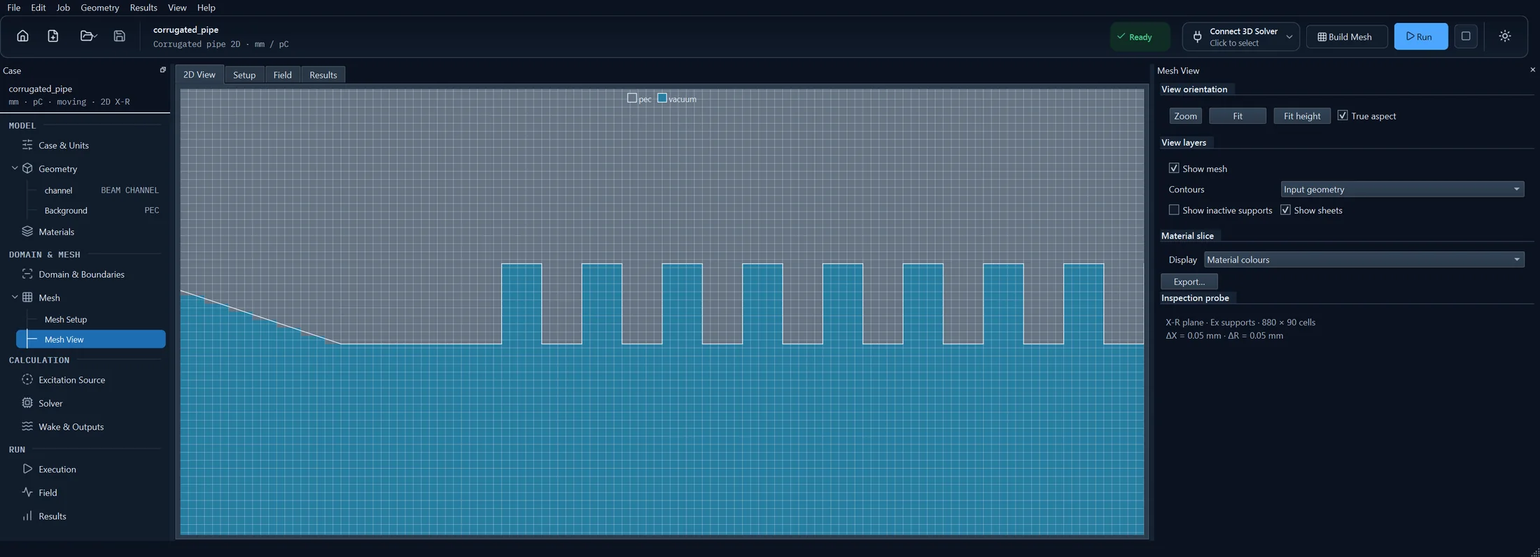
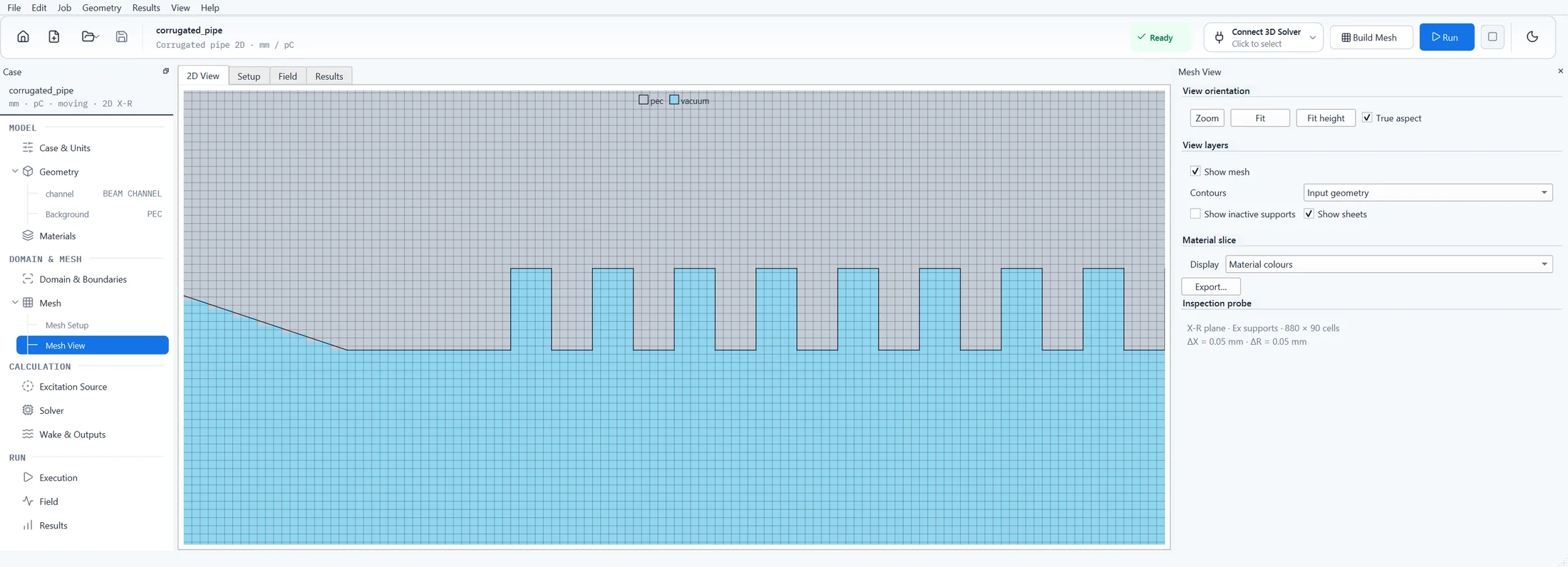
Computed with the 2D Solver. A round corrugated pipe, axisymmetric, azimuthal harmonic m = 0. 1 pC Gaussian bunch, σ = 0.25 mm, β = 1, on axis. Moving window, dispersion-free scheme, mesh 0.05 mm. Field Ex in the plane of axis and radius; the half above the axis is computed and mirrored for the picture. Red is positive, blue negative. A demonstration model.
Geometry
- Lines, circular and elliptical arcs
- Region loops and holes
- Material priorities
- Profile from a STEP model via Studio
Methods
- Stationary and moving grids
- Implicit dispersion-free TE/TM
- Stationary FDTD in selected workflows
- Finite β on stationary grids
Sources
- Gaussian or tabulated bunch
- Several signed sources
- m = 0 and higher azimuthal harmonics
- Analytical width basis for planar models
Walls and materials
- Conducting-wall models
- Layered coatings with backing
- Resistive sheets
- Lorentz dispersion, measured tables
Results
- Physical longitudinal and transverse wakes
- Modal coefficients
- Wakes at new source and witness offsets from saved coefficients
- Per-harmonic diagnostics
- Field recordings
- Loss per family
Execution
- One process, OpenMP threads
- Checkpoint and restart
3D Solver
Computed with the 3D Solver. A dielectric-lined tube: a fused-silica liner (εr = 3.8) in a copper jacket. 1 pC Gaussian bunch, σ = 1 mm, β = 1, on axis. Stationary grid, dispersion-free scheme. Field Ex on the plane through the beam axis; red is positive, blue negative. A demonstration model, not an existing structure.
Geometry and mesh
- STL volume and sheet geometry
- Native analytic and trimmed surfaces from STEP/BREP via Studio
- Background material and overlap priorities
- Conformal Cartesian mesh
- Zero-thickness surfaces
- Longitudinal section templates and repetition
- Mesh reuse
Methods
- Explicit and implicit dispersion-free TE/TM on stationary and moving grids
- Stationary explicit FDTD
- Moving window at β = 1
- Stationary beams with 0 < β < 1
- Open boundaries with PML
- PEC and PMC symmetry planes
Sources and wakes
- One or more transverse point sources with signed charges, common Gaussian σ and β
- Observation trajectories independent of the sources
- Direct and indirect integration
- Dipole output from an opposite-charge pair
Materials and walls
- Vacuum, PEC, linear dielectric and magnetic media, bulk conductivity
- Lorentz dispersion up to ten poles per family
- Measured tables fitted to passive causal models
- Conducting-wall surface models
- Multilayer coatings with PEC, resistive or conducting backing
- Zero-thickness PEC and resistive sheets
- Two-sided layered screens
Losses
- Wall, Ohmic, electric-dispersion and magnetic-dispersion loss
- Total and per material, power and cumulative energy
S-parameters
- Two-port multimode PEC-waveguide scattering
- TE and TM port modes
- Reference-plane de-embedding
- CSV output
Execution
- Hybrid MPI/OpenMP with automatic or explicit Cartesian decomposition
- Checkpoint and restart, also onto a different rank layout
- Slurm submission from Studio
Checks and run times, with their conditions
Models are checked against analytic solutions, mesh refinement and 2D–3D cross-checks; the reports are sent on request. Run times are from an 8-core desktop PC (AMD Ryzen 7 5800X3D, 16 GB, Windows 11) unless stated. Solver versions 1.2.0 (3D) and 0.1.0 (2D) are pre-release builds.
- TESLA cavity with couplers, 3D
Moving window, 0.8 mm mesh, 1,709 steps: solver time 64 s on 6 MPI processes, the largest process using 96 MB. The window holds 3.3 million nodes, where the whole structure would need 50 million. 3D Solver 1.2.0.
- Nine-cell cavity, 2D
Monopole and dipole, 1 mm mesh, 1,166 steps: 9 s including meshing, on 6 threads. Its bunch loss is 1.4 % from the 3D result for the TESLA cavity; the 2D model has no couplers. 2D Solver 0.1.0.
- Dielectric-lined tube, 3D
Stationary grid, 3.24 million cells, 1,962 steps: 165 s on 6 processes. The impedance shows bands at 21.2, about 59 and 97–98 GHz, against 21.1, 58.2 and 98.8 GHz for the TM01, TM02 and TM03 modes of an infinite liner. 3D Solver 1.2.0.
- Corrugated pipe, 2D
Moving window, 79,200 cells, 2,883 steps, monopole and dipole: 18–19 s on 6 threads. The monopole line lies at 91 GHz, against a small-corrugation estimate of 95 GHz. 2D Solver 0.1.0, development build.
- Thin layers and coatings
Coatings and multilayer walls are described by thickness, conductivity, permittivity and permeability, without meshing the layer. A 0.2 µm copper layer is within 3 × 10⁻⁷ of the analytic recursion. Where a slab is meshed, its error falls from 1.8 % to 0.12 % to 0.007 % at 8, 32 and 128 cells in depth; an under-resolved layer is refused.
- Conducting walls
Finite-conductivity walls use a surface model; power lost in walls, conductive volumes and dispersive materials is reported separately. The copper impedance fit is within 1 % from 1 MHz to 5 GHz. In 2D, a resistive pipe is 0.8–1.0 % (L2) from the continuous solution after refinement.
- Dispersive materials
Reflection from a dispersive half-space against the Fresnel formula: the error falls from 4.2 % to 2.1 % to 1.05 % as the mesh is halved twice. 2D against 3D for a ferrite pillbox: bunch loss 0.04 % and magnetic heat 0.07 % apart.
- Open boundaries
Open pipe ends and open transverse boundaries are terminated by perfectly matched layers. A 10-cell transverse layer returns 0.8–1.5 % of the incident amplitude.
- Parallel runs, 3D
The result does not depend on the process layout: differences stay below 10−13 V/pC. A free-space iris on a laptop (Apple M5 Pro, single runs) ran 3.1–3.4 times faster with 4 workers than with one, with per-process memory falling from 435 to 202 MiB. There are no measurements over several cluster nodes.
The TESLA cavity and the corrugated pipe are shown with their fields and wake potentials on the Examples page.
Platforms
Windows x64, macOS on Apple Silicon and Linux. For Linux clusters, packages of the 3D Solver are prepared for specific sites, with Slurm submission from Studio.